Van der Waals Loops and Size Dependence

 Here, building upon previous work[134], we consider the conditions for a Van der Waals loop to occur in the microcanonical caloric curve using a two state model. By differentiating equation 3.30, we obtain

$$\left({\partial T \over \partial E} \right)_{N,V} = T^2 \su... ...} \left({\partial p_i \over \partial E} \right)_{N,V} \right],$$ (3.50)

where the probabilities and their derivatives obey $\sum_i p_i = 1$ and $\sum_i \left(\partial p_i / \partial E \right)_{N,V} =0$.For a two state system, this expression becomes

$$\left({\partial T \over \partial E} \right)_{N,V} = T^2 \le... ...2} \left({\partial T_2 \over \partial E} \right)_{N,V} \right).$$ (3.51)

The first term in this expression is negative and the second positive (assuming region 1 has a lower potential energy than region 2). To exhibit a Van der Waals loop, the caloric curve must have a region of negative slope, and therefore the following inequality must be satisfied for some range of energy,

$$\left({\partial p_2 \over \partial E} \right)_{N,V} \left( {... ...er T_2^2} \left({\partial T_2 \over \partial E} \right)_{N,V} .$$ (3.52)

If we assume both regions behave harmonically, then $\,T_1=\alpha E\,$ and $\,T_2=\alpha (E-\Delta )$, where $\Delta$ is the potential energy difference between the minima of the two regions. This assumption gives

 $$\begin{eqnarray} \left({\partial p_2 \over \partial E} \right)_{N,V} \left( {1 \... ... (p_2 - p_1) + O \left( \left({\Delta \over E} \right)^2 \right). \end{eqnarray}$$

(3.53)




(3.54)

In the middle of the coexistence region where p₁=p₂=1/2, neglecting second order terms in $(\Delta /E)$ gives

$$\left({\partial p_2 \over \partial E} \right)_{N,V} \Delta \gt 1.$$ (3.55)

This equation was previously derived by Bixon and Jortner[152] for Van der Waals loops in the kinetic temperature. We now continue the analysis, first noting that

$$\begin{eqnarray} \left({\partial p_i \over \partial E} \right)_{N,V}&=& {1\over ... ..._{N,V}, \\ &=&{p_i \over k}\left({1 \over T_i}-{1\over T}\right). \end{eqnarray}$$

(3.56)


(3.57)

Therefore, using equation 3.30

$$\left({\partial p_2 \over \partial E} \right)_{N,V}={p_1 p_2... ...right) ={p_1 p_2 \over \alpha k} {\Delta \over E(E-\Delta )}.$$ (3.58)

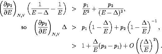
Substituting this result into equation 3.53 and rearranging gives

$$\left(p_1-{p_1 p_2 \over \alpha k}\right) \left({\Delta \over E}\right)^2 - 2 p_1 {\Delta \over E} +1 < 0.$$ (3.59)

Taking the middle of the coexistence region, where p₁=p₂=1/2 and $E=E_\half$:

$$\left(1- {1 \over 2 \alpha k}\right) \left({\Delta \over E_\half}\right)^2 - 2 {\Delta \over E_\half} +2 < 0.$$ (3.60)

As this quadratic has negative curvature for all realistic values of $\alpha$,the above inequality has a physically meaningful solution when $(\Delta / E_\half)$ is greater than the larger root of the quadratic. This solution is

$${\Delta \over E_\half} \gt {\left(\displaystyle{1 \over \alp... ...1/2}-1 \over \left(\displaystyle{1 \over 2 \alpha k}-1\right)}.$$ (3.61)

For a single harmonic minimum of an N-atom cluster

$${1 \over \alpha } =\left({\partial E \over \partial T} \right)_{N,V} = (3 N -7)k.$$ (3.62)

Hence,  

$${\Delta \over E_\half} \gt {2((3N-8)^{1/2}-1) \over (3N-9)}\approx{2 \over \sqrt{3N}}\qquad\hbox{for large }N.$$ (3.63)

A similar relationship can be derived for the N-dependence of Van der Waals loops in the caloric curve of the isopotential ensemble. In this case

$$\left({\partial E_c\over\partial T_c}\right)_{N,V}=\left({3N\over 2} -4\right)k,$$ (3.64)

where E_c is the potential energy and T_c is the isopotential temperature. Hence,

$${\Delta\over E_{c,\half}}\gt 2\sqrt{2\over 3N}\qquad\hbox{for large }N.$$ (3.65)

As $E_{c,\half}<E_\half/\sqrt{2}$, this confirms that a Van der Waals loop is more likely in the isopotential ensemble than the microcanonical ensemble. As we saw earlier, 13 has a Van der Waals loop in the isopotential caloric curve but not in the microcanonical curve.

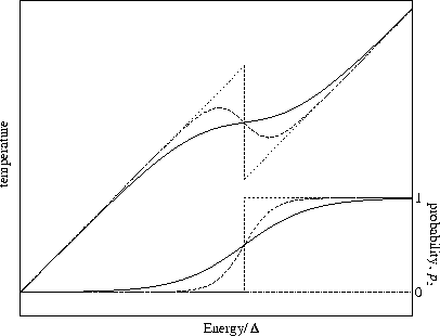
From equation 3.63 it is clear that for a series of structures with similar values of $\Delta/E_\half$, a Van der Waals loop will become more likely as the size increases (Figure 3.16). This result is in good agreement with simulations of icosahedral LJ[135] and cuboctahedral gold clusters[136].

  

Figure 3.16: Plots of temperature (top) and probability, p₂, (bottom) for a two state system. $E_\half/\Delta$ is kept constant as N is varied. The solid line is for small N, long dashed line is for intermediate N and the short dashed line for the bulk limit.

In the bulk limit the above model predicts the caloric curve will be vertical at $E_\half$ (Figure 3.16), which is clearly at variance with the expected behaviour for a bulk first-order phase transition. This discrepancy arises because we have not allowed for the cluster dividing into distinct solid-like and liquid-like regions, which would contribute a term of the form $\Omega_s^{(1-x)}\Omega_l^x$ to the density of states, where x is the fraction of the cluster that is liquid-like. Such phase separation does not occur for small clusters because the energy of the dividing surface makes it unfavourable, but for the bulk the interface is a negligible fraction of the total energy. Recently, an analytical model has been investigated which predicts the size evolution of the microcanonical caloric curve as phase separation becomes possible[176].

Equation 3.63 also shows us that a Van der Waals loop becomes more likely as the quantity $\Delta/E_\half$ increases. We can understand the conditions for this quantity to be large by considering the density of states for each region. For simplicity we do this within the harmonic approximation. We consider region 1 to be made up of n₁ similar geometric isomers (with the same energy, vibrational frequencies and point group), and region 2 of n₂. Each geometric isomer has 2N!/h_i permutational isomers. These assumptions yield

$$\Omega_1={2n_1 N! E^{\kappa-1} \over h_1\Gamma(\kappa)(h\ove... ...^{\kappa-1} \over h_2\Gamma(\kappa)(h\overline\nu_2)^{\kappa}},$$ (3.66)

where h_i is the order of the point group for states in region i. $\Omega_1=\Omega_2$ at $E=E_\half$. Hence,

$${\Delta \over E_{\half}}=\left(1-\left({n_1 h_2 \overline\nu... ...rline\nu_1)^{\kappa} }\right)^{1/\left(\kappa-1\right)}\right).$$ (3.67)

From this expression we can see that $\Delta/E_\half$ increases, making a Van der Waals loop more likely, as region 1 becomes more solid-like (a few high symmetry, rigid states) and as region 2 becomes more liquid-like (many low symmetry, non-rigid states).

Appendix: Thermodynamic Formulae 

APPENDIX: THERMODYNAMIC FORMULAE

In this appendix, the formulae for some of the thermodynamic quantities that can be calculated by the superposition method are given. The thermodynamic functions are derived from the following definitions.

In the isopotential ensemble,

$$p_i(E_c)={\Omega_{c,i}(E_c)\over \Omega_c(E_c)},\qquad\qquad... ..._c)}=\left({\partial\ln\Omega_c\over\partial E_c}\right)_{N,V}.$$

In the microcanonical ensemble,

$$p_i(E)={\Omega_i(E)\over\Omega(E)}.$$

In the canonical ensemble,

$$p_i(T)={Z_i\over Z},$$

$$U(T)=-\left(\partial\ln Z\over\partial\beta\right)_{N,V} ={1\over Z_{0,0}}(Z_{1,0}+Z_{0,1}),$$

$$\begin{eqnarray} C_v(T)&=&\left({\partial U\over\partial T}\right)_{N,V},\nonumb... ...})-\left({Z_{1,0}+Z _{0,1}\over Z_{0,0}}\right)^2\right),\nonumber\end{eqnarray}$$

$$A(T)=E^0_0-kT\ln Z,$$

$${\cal P}(E)=\Omega(E)\exp(-\beta E),$$

$$A_L(E_c)=E_c-kT\ln\Omega_c(E_c),$$

where in $Z_{\alpha,\delta}$ the derivative of the exponential function of $\beta$in Z has been taken $\alpha$ times and the derivative of the inverse power of $\beta$ in Z $\delta$ times. Therefore, Z=Z_0,0.

Below, we give the thermodynamic functions for the $\gamma$ formulation with a first-order anharmonic correction which was used for 55.

$$T_c(E_c)={\displaystyle\sum_{E_s^0<E_c}\gamma(E')_s\sum_{l=0... ...^\kappa_l a_s^l (E'-E^0_s)^{\kappa+l-1}\over\Gamma(\kappa+l)}}.$$

$$Z _{\alpha,\delta}=c\sum_s\gamma(E')_s(E^0_s)^\alpha e^{-\be... ...C^\kappa_l a_s^l (E'-E^0_s)^{\kappa+l-1}\over\Gamma(\kappa+l)}.$$

$$A_L(E_c)=E_c-{1\over\beta}\ln {c\over\beta^{\kappa/2}} \sum_... ...C^\kappa_l a_s^l (E'-E^0_s)^{\kappa+l-1}\over\Gamma(\kappa+l)},$$

where

$$c={n^*_0\over\gamma(E')_0\prod_{j=1}^\kappa h\nu^0_j}\sum_{l... ...C^\kappa_l a_0^l (E'-E^0_0)^{\kappa+l-1}\over\Gamma(\kappa+l)}.$$

The harmonic forms can be recovered by taking the l=0 term. We obtain the n^* formulation by replacing

$$c\,\gamma(E')_s \bigg/ \sum_{l=0}^\kappa {C^\kappa_l a_s^l ... ...quad\hbox{with}\qquad {n^*_s \over\prod_{j=1}^\kappa h\nu_j^s}.$$

Below, we give the thermodynamic functions for the n^* formulation with second-order anharmonic corrections which was used for 13.

$$T_c(E_c)={\displaystyle\sum_{E_s^0<E_c}{n^*_s \over\prod_{j=... ...} (E_c-E^0_s)^{\kappa/2+l+2m-2} \over\Gamma(\kappa/2+l+2m-1)}},$$

$$Z_{\alpha,\delta}=\sum_{s}{n^*_s e^{-\beta E_s^0} (E^0_s)^\a... ...D^\kappa_{l, m} 3^m a_s^{l+2m}\over\beta^{\kappa+l+2m+\delta}},$$

$$A_L(E_c)=E_c-{1\over\beta}\ln \sum_{E_s^0<E_c}{n^*_s \over\b... ...l+2m} (E_c-E^0_s)^{\kappa/2+l+2m-1}\over\Gamma(\kappa/2+l+2m)}.$$

The harmonic forms can be recovered by taking the l=0, m=0 term, and the first-order correction forms by taking the m=0 terms. We obtain the $\gamma$ formulation by replacing

$${n^*_s \over\prod_{j=1}^\kappa h\nu_j^s} \qquad\hbox{with}\q... ..._s^{l+2m} (E'-E^0_s)^{\kappa+l+2m-1} \over\Gamma(\kappa+l+2m)},$$

where

$$c={n^*_0\over\gamma(E')_0\prod_{j=1}^\kappa h\nu^0_j} \sum_{... ..._0^{l+2m} (E'-E^0_0)^{\kappa+l+2m-1} \over\Gamma(\kappa+l+2m)}.$$