


Next: Van der Waals Loops
Up: Thermodynamics of Small Lennard-Jones
Previous: The effect of well
Home: Return to my homepage
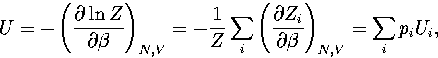
The accurate expressions for  developed in the previous section can be
used to give a wide range of thermodynamic functions,
in fact, all except those that depend on derivatives of N or V.
The exceptions arise because the thermodynamic properties of small clusters are
discontinuously dependent on N and because the volume of a cluster is
hard to define[172]. The formulae for the
functions illustrated in this section are given in the appendix.
They have, for the most part, been derived
in previous work within the harmonic approximation[153,133];
the extension to incorporate anharmonicity follows simply from the
expressions given in the previous section.
The results are given for the most accurate partition functions:
the first-order corrected
developed in the previous section can be
used to give a wide range of thermodynamic functions,
in fact, all except those that depend on derivatives of N or V.
The exceptions arise because the thermodynamic properties of small clusters are
discontinuously dependent on N and because the volume of a cluster is
hard to define[172]. The formulae for the
functions illustrated in this section are given in the appendix.
They have, for the most part, been derived
in previous work within the harmonic approximation[153,133];
the extension to incorporate anharmonicity follows simply from the
expressions given in the previous section.
The results are given for the most accurate partition functions:
the first-order corrected  formula for LJ55 using sample A and the
second-order corrected n* formula for LJ13 using sample D.
formula for LJ55 using sample A and the
second-order corrected n* formula for LJ13 using sample D.
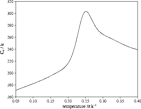
Figure 3.9:
Comparison of harmonic and anharmonic thermodynamic functions of LJ55:
(a) the microcanonical (solid line) and canonical (dashed line) caloric curves,
(b) the isopotential caloric curve, (c) Cv(T) and (d) A(T).
In all except (a) the anharmonic curve is denoted by a solid line and the harmonic by a dashed line.
Energies are measured with respect to the global minimum icosahedron.
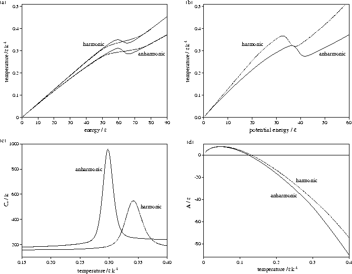 |
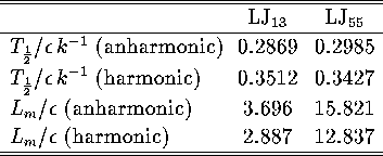
Harmonic and anharmonic results for the caloric curves, the heat capacity Cv,
the Helmholtz free energy A, the transition temperature  and the latent heat Lm
are compared in Figures 3.9 and 3.10 and Table 3.8.
We define as the temperature for which the two states have an
equal Landau free energy, AL(Ec).
Lm is the internal energy difference between the two states at and was obtained by extrapolating the caloric curves for each state
to using equation 3.29. For LJ13, this procedure simply gives
and the latent heat Lm
are compared in Figures 3.9 and 3.10 and Table 3.8.
We define as the temperature for which the two states have an
equal Landau free energy, AL(Ec).
Lm is the internal energy difference between the two states at and was obtained by extrapolating the caloric curves for each state
to using equation 3.29. For LJ13, this procedure simply gives
 ,
where Ui is the internal energy of region i.
For LJ55, we have used
,
where Ui is the internal energy of region i.
For LJ55, we have used  , where
  is the internal energy for the region of the PES
formed from the combination of regions
1-4,
and so Lm does not include the latent heat associated with the
disordering of the surface that occurs before melting.
Just integrating Cv over the transition region would overestimate Lm
because it would also include the energy needed to raise the temperature of the cluster.
is the internal energy for the region of the PES
formed from the combination of regions
1-4,
and so Lm does not include the latent heat associated with the
disordering of the surface that occurs before melting.
Just integrating Cv over the transition region would overestimate Lm
because it would also include the energy needed to raise the temperature of the cluster.
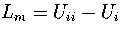
Figure 3.10:
Comparison of harmonic and anharmonic thermodynamic functions of
LJ13: (a) the microcanonical (solid line) and canonical (dashed line) caloric
curves, (b) the isopotential
caloric curve, (c) Cv(T) and (d) A(T). In all except (a) the anharmonic
curve is denoted by a solid line and the harmonic by a dashed line. Energies
are measured with respect to the global minimum icosahedron.
 |
Table 3.8:
Transition temperatures and latent heats for LJ13 and LJ55.
 |
The anharmonic caloric curves are displaced downward and
away from their harmonic equivalents because of the increased densities of
states associated with higher potential energy, lower temperature regions of
the PES. The anharmonic heat capacity curve of LJ55 is in very good agreement with
results from the multi-histogram MC[135] and J-walking[173] simulations.
The peak in the heat capacity curve is larger and sharper when
anharmonicity is included. This change can be understood by considering a two level system,
which is a reasonable model to describe the equilibrium
between solid-like and liquid-like states of the cluster.
The partition function can be written as  , where the sum is
over the two distinct regions of phase space.
It follows that
, where the sum is
over the two distinct regions of phase space.
It follows that
|  |
(3.40) |
where pi=Zi/Z and 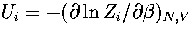 .
Hence,
.
Hence,
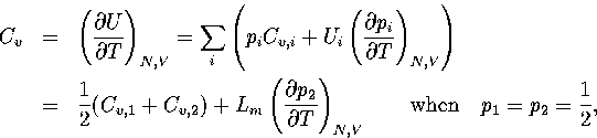
(3.41)
(3.42)
where 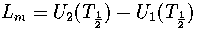 and
and  .As
.As
|  |
(3.43) |
(3.44)
(3.45)
Substituting this result into equation 3.42 gives
|  |
(3.46) |
The greater anharmonicity of liquid-like minima causes Lm to be larger when
anharmonicity is included. This change has two effects: it increases the area under
the heat capacity peak, and causes the cluster to change between the two states more
rapidly with temperature, decreasing the width of the peak.
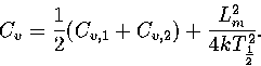
Figure 3.11:
Probabilities of LJ55 being in regions I,
II, III,
IV and VI
of the PES for (a) canonical, (b) microcanonical and (c) isopotential ensembles.
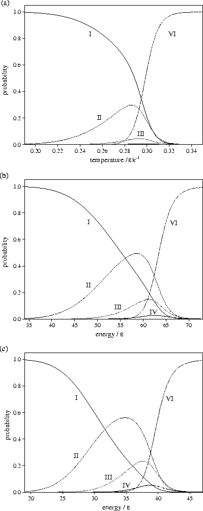 |
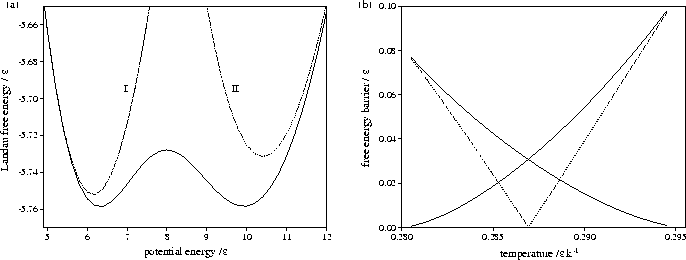
Figure 3.12:
Plots for LJ55 of (a)  at T=0.2985, (b) AL(Ec) at T=0.2985
(c) AL(Ec) at a number of temperatures as labelled and
(d) the free energy barrier heights (solid lines) and the free energy difference between solid-like
and liquid-like states (dashed line) for AL(Ec). In (a) and (b)
the contributions of the different regions of the PES are also indicated.
In (c) the results from our analytic partition function (solid line) are compared to
simulation results (data points)[133].
at T=0.2985, (b) AL(Ec) at T=0.2985
(c) AL(Ec) at a number of temperatures as labelled and
(d) the free energy barrier heights (solid lines) and the free energy difference between solid-like
and liquid-like states (dashed line) for AL(Ec). In (a) and (b)
the contributions of the different regions of the PES are also indicated.
In (c) the results from our analytic partition function (solid line) are compared to
simulation results (data points)[133].
 |
From Figure 3.11 it can be seen that the probability of LJ55 being in
regions 2 and 3
is lowest in the canonical ensemble and highest in the isopotential ensemble. This
result is due to the dependence of the partition function on the independent variables,
T, E and Ec, of the three ensembles. In the canonical ensemble, Z is exponentially dependent
on T, and is the most steeply varying of the three partition functions. In the microcanonical
and isopotential ensembles,  and
and  are dependent on powers of E and Ec,
respectively. As the exponent of Ec is lower than that for E, is the slowest varying
of the partition functions.
For LJ55
are dependent on powers of E and Ec,
respectively. As the exponent of Ec is lower than that for E, is the slowest varying
of the partition functions.
For LJ55  (Table 3.9), where
  ,
,
 and
and  are the number of minima in regions
1,
2-3
and 6, respectively.
Consequently, as the partition function becomes more steeply varying,
the defective icosahedra are seen for a narrower range of the independent variable,
i.e. the contribution of the liquid-like states overtakes the defective icosahedra
at an earlier stage in the generation of surface defects.
are the number of minima in regions
1,
2-3
and 6, respectively.
Consequently, as the partition function becomes more steeply varying,
the defective icosahedra are seen for a narrower range of the independent variable,
i.e. the contribution of the liquid-like states overtakes the defective icosahedra
at an earlier stage in the generation of surface defects.
Figure 3.13:
Plots for LJ13 of
(a) AL(Ec) at T=0.2869, and
(b) the free energy barrier heights (solid lines) and
the free energy difference between solid-like and liquid-like states (dashed line) for AL(Ec). In (a) the
contributions of liquid-like and solid-like states are shown.
 |
The Landau free energy, AL(Q), is the free energy of a system for a particular value of an order parameter Q.
It is defined by
| 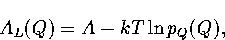 |
(3.47) |
where pQ(Q) is the canonical probability distribution of the order parameter.
The presence of two minima in AL(Q) indicates that there are two thermodynamically
stable states at this temperature.
As A is independent of Q, knowledge of pQ(Q) is sufficient to calculate the Landau free energy barrier.
When Ec is used as an order parameter, simulations have shown that LJ55 has two Landau free
energy minima which correspond to the solid-like and liquid-like states[133].
Bimodality in the canonical energy distribution function, ,
implies that there are two Landau free energy minima as a function of the order parameter, E.
Figures 3.12 and 3.13 show that both LJ13 and LJ55 have a range of temperature for
which two Landau free energy minima are observed.
As can be seen from 3.12c the predicted free energy curves for LJ55
are in very good agreement with those from simulation[133], confirming the
accuracy of our analytic partition function.
The states corresponding to the Mackay icosahedron and the defective icosahedra all
contribute to the low potential energy minimum of AL(Ec),
but the free energies of regions IV and
V are never low enough to affect the thermodynamics.
Although the free energy barrier for LJ13 is much smaller,
it has been observed in some simulations[142,174].
The turning points in AL(Ec) and correspond to points on the
isopotential and the microcanonical caloric curves, respectively.
This can be demonstrated for AL(Ec) by solving the equation  .The solution is
  , which is simply the definition of the
isopotential temperature.
The maxima in AL(Ec) correspond to the segment of the caloric curve with negative slope, and
the minima to segments with positive slope.
Therefore the temperature range for which AL(Ec) has two minima is the same as the depth of the
Van der Waals loop in the isopotential caloric curve, as can be seen by comparing
Figures 3.9b and 3.12d, and 3.10b and 3.13b.
, which is simply the definition of the
isopotential temperature.
The maxima in AL(Ec) correspond to the segment of the caloric curve with negative slope, and
the minima to segments with positive slope.
Therefore the temperature range for which AL(Ec) has two minima is the same as the depth of the
Van der Waals loop in the isopotential caloric curve, as can be seen by comparing
Figures 3.9b and 3.12d, and 3.10b and 3.13b.
Comparing the results for LJ13 and LJ55 the effects of size are apparent.
For LJ55 the melting transition is much more pronounced: it has a sharper
peak in Cv, more pronounced Van der Waals loops in the microcanonical and isopotential
caloric curves, a larger Landau free energy barrier, a larger temperature
range for which solid-like and liquid-like clusters coexist, a larger latent
heat per atom and a higher melting temperature.
This behaviour is closer to the first-order phase transition of bulk matter.
Figure 3.14:
Heat capacity of LJ55 when only regions V and
VI are included in the partition function.
 |
One feature of the superposition method is that it allows one to restrict the regions of configuration space considered,
and hence to look at thermodynamic properties which would be difficult to obtain by other methods.
For example, we can study the thermodynamic effects of structural relaxation in the absence
of a transition to the solid-like state, thus enabling us to study supercooled liquid-like
and perhaps even glass-like clusters.
This could not easily be done by simulation since for LJ55 the cluster readily
passes into the solid-like region of configuration space on cooling.
Shown in Figure 3.14 is
 ,
the heat capacity when only regions 5 and 6
are included in the partition function.
It shows a clear peak at T=0.252 (0.84),
which has a height above the background Cv that is about a seventh of that for melting.
It resembles the heat capacity peak that is often seen at the bulk glass transition.
Such an interpretation should be caveated by the fact that the peak is dependent on where one
decides the low energy tail of the liquid-like minima finishes.
,
the heat capacity when only regions 5 and 6
are included in the partition function.
It shows a clear peak at T=0.252 (0.84),
which has a height above the background Cv that is about a seventh of that for melting.
It resembles the heat capacity peak that is often seen at the bulk glass transition.
Such an interpretation should be caveated by the fact that the peak is dependent on where one
decides the low energy tail of the liquid-like minima finishes.
Figure 3.15:
Plot of Gm(Ec) for LJ55 as a function of the potential energy
calculated using sample B.
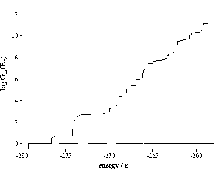 |
Estimates of the number of minima in different regions of the PES can be
obtained from the quench frequencies.
Using equations 3.6, 3.7 and
3.9 an expression for gs can be derived:
|  |
(3.48) |
From gs, the sum of minima, Gm(Ec),
can easily be calculated
|  |
(3.49) |
This approach has been applied to LJ55.
From Figure 3.15 it can be seen that above  the number
of minima rises exponentially with the energy.
The total number of minima in the energy range probed by the MD quenching
(potential energies up to
the number
of minima rises exponentially with the energy.
The total number of minima in the energy range probed by the MD quenching
(potential energies up to  ) is
) is  .This value is much less than the total number of minima
predicted by extrapolating Tsai and Jordan's results for small clusters and
so suggests that the number of minima will continue to rise exponentially above .The present method has also been used to estimate the number of minima in the energy ranges
I-VI (Table 3.9).
The number of minima in range
II is known[108] to be 11.
The results from the
quench frequencies agree well with this figure.
.This value is much less than the total number of minima
predicted by extrapolating Tsai and Jordan's results for small clusters and
so suggests that the number of minima will continue to rise exponentially above .The present method has also been used to estimate the number of minima in the energy ranges
I-VI (Table 3.9).
The number of minima in range
II is known[108] to be 11.
The results from the
quench frequencies agree well with this figure.
Table 3.9:
Estimated numbers of geometrically distinct minima of LJ55 in the
six energy ranges given in Table 3.1 calculated using sample A.
| Region |
number of |
minima |
| |
anharmonic |
harmonic |
| I |
1 |
1 |
| II |
11.3 |
6.3 |
| III |
994.6 |
457.9 |
| IV |
81.5 |
2871.2 |
| V |
 |
 |
| VI |
 |
 |
The methods developed here should be applicable to other types of clusters,
although, as in our examples, the most appropriate form for the anharmonic terms
may depend on the type and size of cluster considered.
The advantages of the superposition method are that once the partition function
is obtained it can be used to calculate a whole gamut of thermodynamic properties analytically,
and that it allows one to consider the roles of different regions of configuration
space and so gain more physical insight into the system, particularly the
relationship between structure and thermodynamics.
(If one simply wants without these extras, one should use
a simulation method, such as multi-histogram MC[141].)
However, the method currently relies upon there being an energy at which all
relevant regions of phase space are sampled.
This condition does not hold for larger clusters, such as LJ147.
To extend the method to such systems an analogue of the multi-histogram technique
would need to be developed, in which the information from quenching at different
energies could be combined.
The expressions for the density of states could also be used to calculate accurate rate
constants using RRKM (Rice-Ramsperger-Kassel-Marcus) theory[166,175],
and so aid quantitative elucidation of dynamic properties
from a knowledge of the transition states on the PES.
Next: Van der Waals Loops
Up: Thermodynamics of Small Lennard-Jones
Previous: The effect of well
Home: Return to my homepage
Jon Doye
8/27/1997