 |
(5.1) |
If the transition matrix w is neither decomposable nor splitting,
the matrix has a single zero eigenvalue[255],
whose eigenvector corresponds to the equilibrium probability distribution, ![]() .
The master equation describes the evolution of a system from an initial distribution,
.
The master equation describes the evolution of a system from an initial distribution, ![]() ,towards
,towards ![]() ;at infinite time the probability distribution
must be equal to
;at infinite time the probability distribution
must be equal to ![]() .The dynamics and thermodynamics must be consistent in this limit.
.The dynamics and thermodynamics must be consistent in this limit.
The transition matrix must satisfy detailed balance
to be physically reasonable, i.e. WijPeqj=WjiPeqi.
As a consequence, the solution of the master equation can be expanded in a complete
set of eigenfunctions of the symmetric matrix, ![]() , defined as
, defined as
![]() . The result is[254]
. The result is[254]
 |
(5.2) |
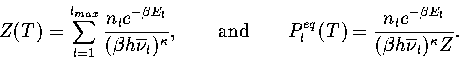
The concept of detailed balance also allows us to define when two states
come into local equilibrium; i.e. ![]() .
The precise condition that we use is
.
The precise condition that we use is
 |
(5.3) |
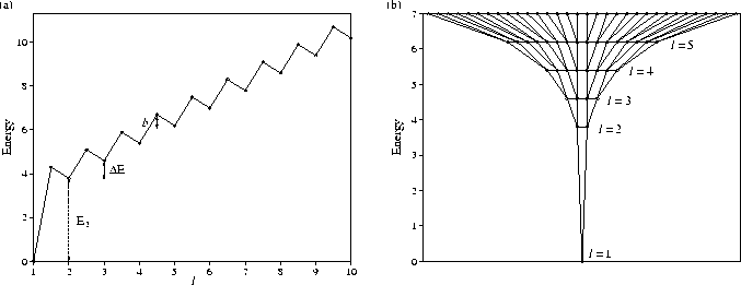 |
The standard PES that we consider is depicted in Figure 5.1.
It consists of a single funnel in which the number of minima increases rapidly
with energy (Figure 5.1b).
To simplify the calculations the minima have been grouped into lmax levels.
The minima in each level are assumed to have identical properties, and to be always in
equilibrium with each other, thus allowing us
to consider each level as a single state in the master equation.
This framework is equivalent to assuming that the barriers between minima
in the same level are zero. Level l=1 is the global minimum, and
the number of minima increases geometrically as the PES is ascended. There are g times more
minima in each subsequent level. Therefore the number of minima in level l, nl, is gl-1
and the total number of minima on the PES is (glmax-1)/(g-1).
We do not consider permutational isomers explicitly
since they do not affect the relaxation dynamics.
For a real PES, there are ![]() permutational isomers of each minimum.
Therefore, there will be many funnels leading down to the different
permutational isomers of the global minimum.
However, as each funnel is identical they do not need to be considered separately.
permutational isomers of each minimum.
Therefore, there will be many funnels leading down to the different
permutational isomers of the global minimum.
However, as each funnel is identical they do not need to be considered separately.
We assume that the minima in level l are only connected to minima in levels ![]() .
The transition states connecting minima in adjacent levels are all assumed to lie an energy
b above the higher minimum.
Each minimum in level l is assumed to be connected to
.
The transition states connecting minima in adjacent levels are all assumed to lie an energy
b above the higher minimum.
Each minimum in level l is assumed to be connected to ![]() minima in level l-1 and hence
to
minima in level l-1 and hence
to ![]() minima in level l+1.
From this information, and using RRKM theory[166]
within the harmonic approximation, the microcanonical rates for transitions between levels are
minima in level l+1.
From this information, and using RRKM theory[166]
within the harmonic approximation, the microcanonical rates for transitions between levels are
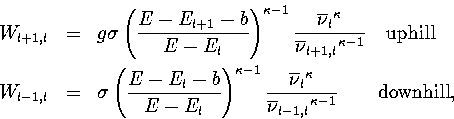
(5.4)
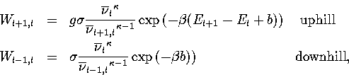
(5.5)
The thermodynamics of the system can be described using a superposition method (Chapter 3),
whereby the total energy density of states, ![]() , is constructed by summing the density of
states for all the energetically accessible minima on the PES.
Applying this method to the model PES within the
harmonic approximation gives
, is constructed by summing the density of
states for all the energetically accessible minima on the PES.
Applying this method to the model PES within the
harmonic approximation gives
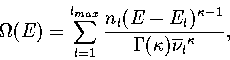 |
(5.6) |
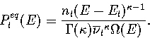 |
(5.7) |
 |
(5.8) |
The global minimum defines the energy zero, i.e. E1=0. Beyond l=2
the potential energy is assumed to increase linearly with l.
Therefore, ![]() for
for ![]() , where
, where ![]() is a measure
of the potential energy gradient of the funnel.
For a typical cluster PES, the mean vibrational frequency is smaller for minima
of higher potential energy[153]--the stabilization of the liquid-like phase at
high temperatures is due to both the large number of minima and the greater
vibrational entropy. Therefore, we use
is a measure
of the potential energy gradient of the funnel.
For a typical cluster PES, the mean vibrational frequency is smaller for minima
of higher potential energy[153]--the stabilization of the liquid-like phase at
high temperatures is due to both the large number of minima and the greater
vibrational entropy. Therefore, we use
![]() This defines the unit of time as the vibrational period of the global minimum.
The mean vibrational frequency of a transition state is assumed to be the geometric mean
of the vibrational frequencies of the two minima it connects,
i.e.
This defines the unit of time as the vibrational period of the global minimum.
The mean vibrational frequency of a transition state is assumed to be the geometric mean
of the vibrational frequencies of the two minima it connects,
i.e. ![]()